Go back to Decisions and Calculations
Chapter 08: Instantiation
Like functions and function calls, instantiation is one of the most important concepts in programming. And even though we have seen examples of instantiation before, I want to spend a whole chapter to drill the idea into you.
Instantiation recapped
So let us recap what we have seen of instantiation so far, and try to define the idea as we go along. Consider the following program:

The thing after the colon is the (explicitly given) type of the value v.
The literal 10 is the value. We could have written
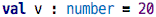
as well. So both 10 and 20 have type number, otherwise we could not
legally write this code. The notion of instantiation is actually the
inverse relationship of “has type”. So instead of saying that 10 and 20
have type number, we could say that these two are both instances
of the type number. Values are instances of types.
Let us go back to records:
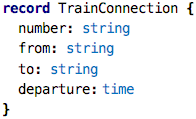
This example captures the notion of a train connection (guess where I am writing this :-)). We can create values of this type, i.e., record instances by writing

So what is different here compared to the number examples above? We
provide values for each of the members of the record. So here, the type
can be seen as a kind of template for constructing values. The template
defines “holes”, i.e., things that an instance can define freely when they
are created. So different instances can be distinguished by the values they
have for the “holes”.
The type defines which values are valid for instances. Let’s look at this statement a little bit more closely by looking at the following examples:
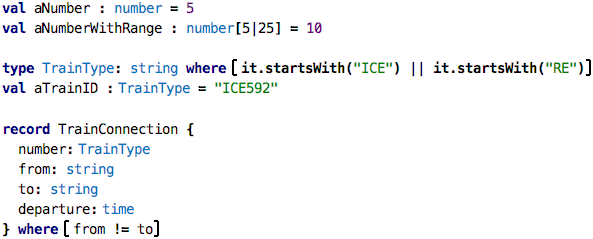
The first one defines a number without any further constraint (although
we know that if we don’t specify a precision, no decimal digits are allowed,
so this is a kind of implicit constraint). The aNumberWithRange is more picky,
because the range specified on the type is of course a constraint on the
set of allowed values. The next example defines a new type based on the
string type. That new type, TrainType, has a constraint that expresses
that valid values have to begin with the string ICE or RE (two kinds
of trains in Germany, InterCity Express and Regional Express). You can express
a constraint on any type using the where keyword. For example, you could
define the type of odd numbers as type oddNum : number where isOdd(it).
Finally, the new version of the TrainConnection defines a constraint that
expresses that the train cannot arrive in the same city from which it
leaves. We get errors when we try to create instances that do not
conform to these rules, which is why all the following tests fail.
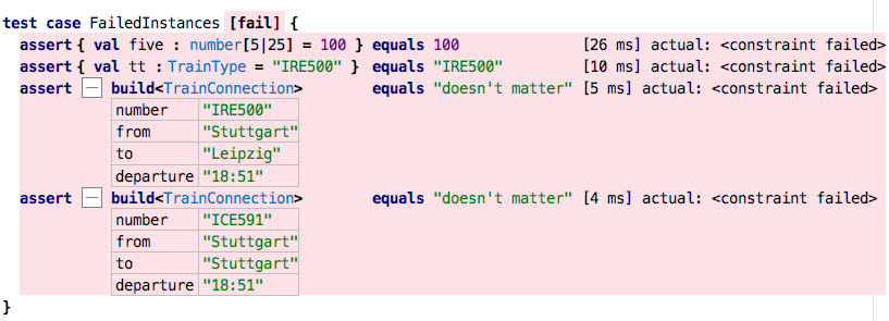
Failing tests are bad. Always. So, can we write a test that expects the constraints to fail (and then becomes green)? Yes, we can:
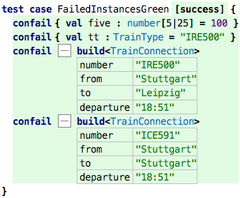
Constraints expressed this way are checked at runtime, we have to actually run the tests. Checking them in the type system is too complicated. The only exception is the number ranges; here, the IDE actually reports an error as soon as you write the program.
Ok, so this is essentially a recap of what we have seen so far: instances are values that have a particular type, that provide values for the “holes” left open by the type, if any, and respect the constraints expressed by the type, implicitly or explicitly. Let’s look at more examples of this.
Sheet Templates
Can we play with the idea of instantiation in Spreadsheets? What would this mean? Look at the following example:
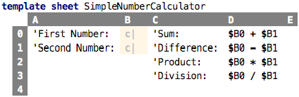
This sheet computes the sum, difference, product and division of two numbers.
The particular numbers for which it does this are not specified. However,
this is a template sheet, i.e., a sheet that is intended for instantiation;
the two values that are used for the computations are the “holes” in the
type, i.e., they are specified in instances. For the expressions in the
D column to type check, we have to give a type for the unspecified values
in column B. And in fact, the two cells there are constrained, as indicated
by the little c and the yellowish background color. If we show the sheet
in a slightly different way, we can see the constraints:
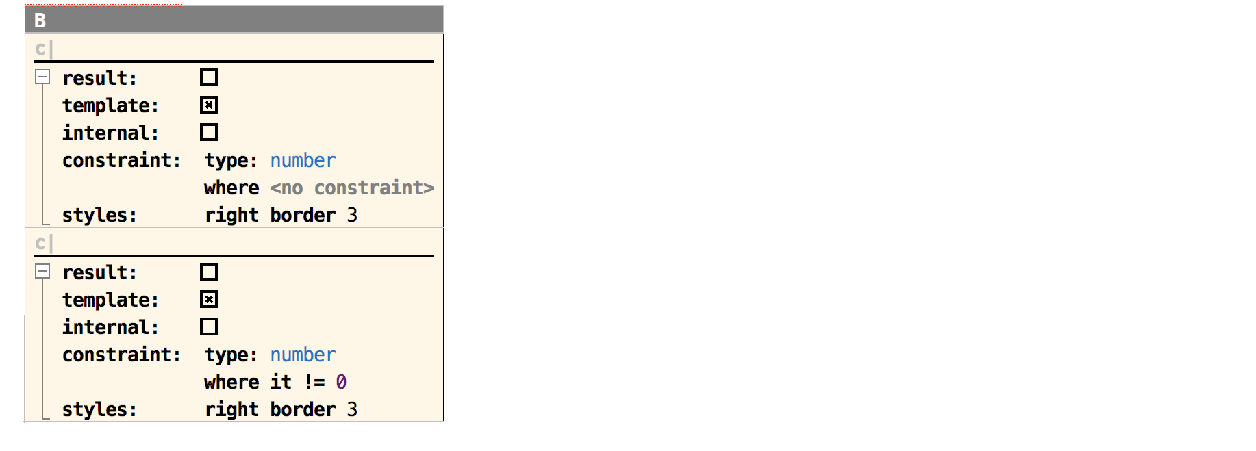
We define the type to be number for both, and for the second one
we even express that the value cannot be zero, because otherwise we’d run
into a division by zero when we divide the two numbers in cell D3.
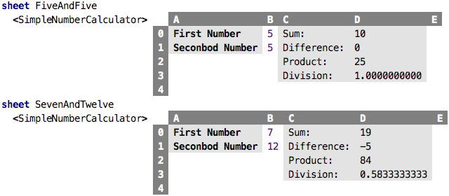
So, let’s create an instance:
As you can see, it is automatically shown in “value mode”, where all the expressions are already evaluated. No values have been provided for the two numbers in column B so far. So it is actually an invalid instance. Let’s provide values:
Why did I show this example? I want to drive home the idea almost anything can be made into a type, and thus be made instantiatable. Just leave holes, let instances fill values for the holes, and check the hole-values provided by the instances against the constraints specified by the type. That’s it!
Usually an instance retains a reference to its type. In records, notice how an instance
#Person{"Markus", "Voelter"}references the recordPerson. Similarly, the spreadsheet instances shown above also refer to the template spreadsheet in between the angle brackets. This is so we can check the conformance of the instance against its type.
Data Flow Blocks
If you are a “business person” you probably find the spreadsheet-based examples intuitive because of your experience with Excel. If you are an engineer, you probably want to see block diagrams. But even if you’re not an engineer, you will learn quite a bit from this example as well. Take a look at the following code:
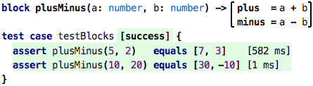
A block is a new abstraction, you can see it as a function that has
more than one result. The plusMinus block takes two numbers, and
returs two results: the plus result where a and b are added,
as well as the minus result that subtracts the two. The two results
are computed separately, just as if it were a function with two bodies.
So nothing really new here. In fact, if you think about it, it’s really
almost exactly the same as the instantiatable spreadsheet example: we
also calculated several values (sum, difference, product, division) for
the same set of inputs.
You can also call a block as if it were a function. However, as we know, functions have only one result. How can we package two results into one? We could use a list, or a record, or something we have not seen before, a tuple:
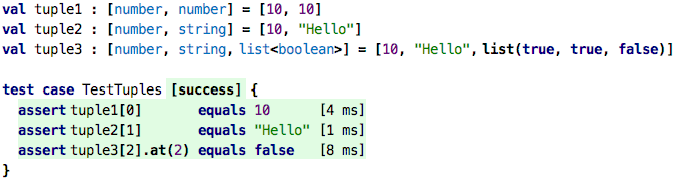
Tuple types are lists of types enclosed in square brackets, and the
values are written using the same notation, of course now as a list of
comma-separated expressions. When you have a tuple value in your hand,
you can use the [] notation to access the tuples’ elements by position.
So, as a brief recap, here’s a comparion between records, lists and tuples:
| Record | List | Tuple | |
| Number of Elements | Fixed | Variable | Fixed |
| Are elements named? | Named | Anonymous | Anonymous |
| All elements same type? | Different Types | Same Type | Different Types |
| Explicitly declared and named? | Declared | Anonymous | Anonymous |
So, returning to our blocks, the expression plusMinus(5, 2) in the test case
calls a block, and receives the two results as a tuple. We express the expected
result as a tuple as well. Here is this initial example again:
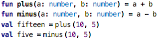
Let us define a few more blocks:
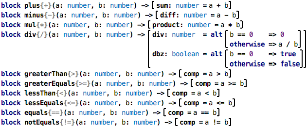
As you can see, these blocks essentially wrap the basic arithmetic and comparison
operators we have used before. Most of them have exactly one output, except the
div block, which also outputs if a division by zero would have occured because
the second argument was zero.
So what is the point of this exercise? These blocks can be used for graphical programming, where we draw diagrams that represent block instances and the flow of data between them. We package such diagrams into yet other blocks, so-called composite blocks, which can then be instantiated further. Let’s illustrate this.
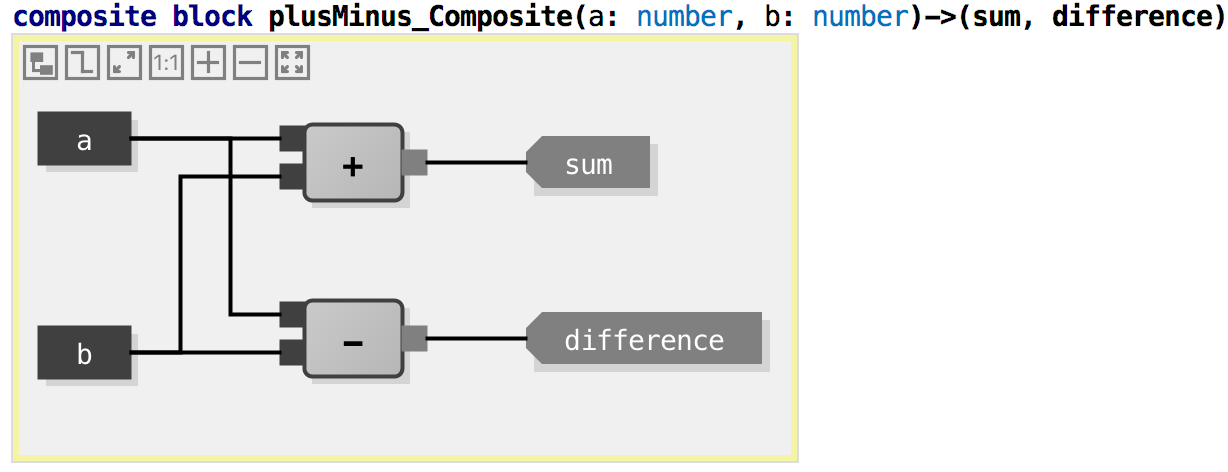
This graphical notation works as follows. The dark rectangles on the left (a, b) are
inputs of the current block. The gray boxes with diagonal corners (sum, difference)
are outputs of the block. These are read-only, graphical representations of the block’s interface that is defined textually in the header of the block:

The rest of the diagram, i.e., in this example, the + and - block instances
and the connections, are done graphically. You drag and drop blocks from the palette, and then draw the connectors using the mouse:
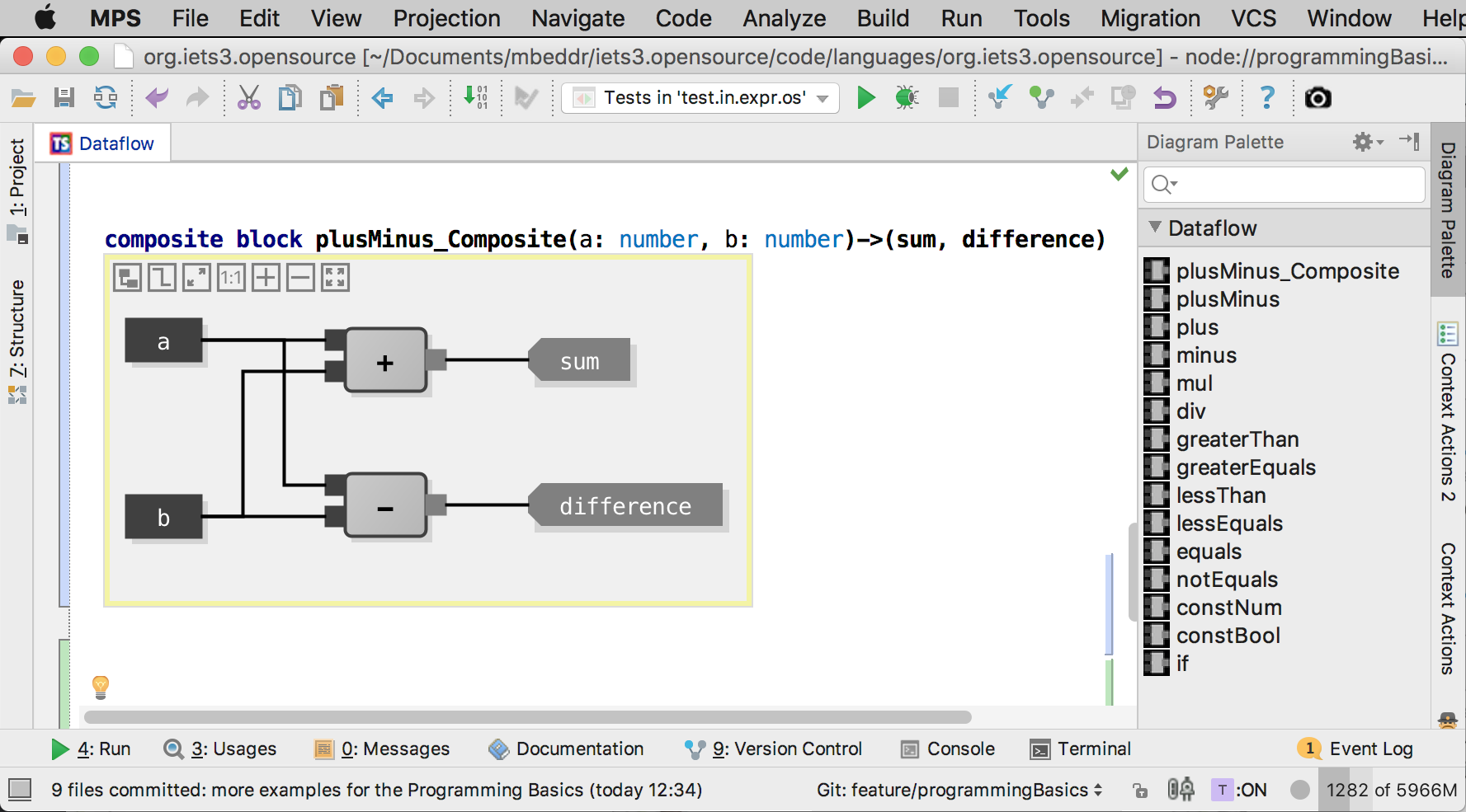
So what exactly are we seeing here? The grey rectangles are instances of
previously defined blocks; the symbols are defined with the block, see the
set of predefined blocks above. The lines represent the data flow. In this
example, the data flows from the inputs (a, b) to the two inputs of the
instances inside this composite block. So, as the name suggests, this block
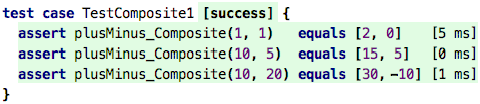
computes the sum and difference of the two inputs. Let’s verify the behavior
via a few tests:
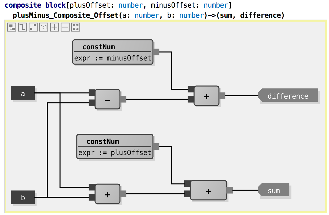
Let’s make this a little bit more complicated: both the sum and the difference
can now be offset by a constant value each. We use the constNum block which simply
outputs the number that is given to it by the configuration parameter expr.
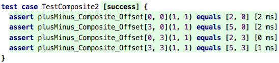
Let’s write tests:
To return to the discussion about instantiation: this composite block
contains several instances of other blocks: 3 of the block +, two of
the block constNum, and one of the block -. The composite block
can of course also be instantiated:
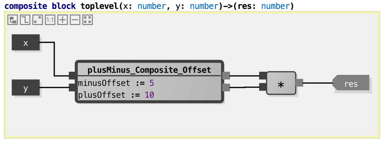
Here we have instantiated the composite block from above into a new
composite block. Of course, once we do this, we have to specify the two
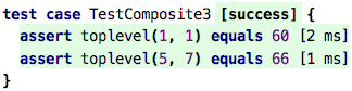
parameter values (offsetPlus, offsetMinus). To compute one single
result, we multiply the sum and the difference. Tests:
So what is good and bad about this? What is good is that this approach supports nice modularization – by packaging functionality into reusable blocks, we can reuse – reinstantiate – those blocks in different context. Modularization is generally good, and we will discuss it much more in later chapters.
What about the graphical notation? Generally, people tend to like graphical notations: “a picture says more than 1000 words”. However, let’s be realistic: it also takes up a lot of space, and visually following a network of black lines is not necessarily simpler than working with names (if we were to use functions instead of blocks). So how would this same behavior look like if we were to use plain functions? Here is the code if we retain the nesting structure, i.e., each block becomes a function, each instance becomes a function call, and each line becomes a use of a parameter:
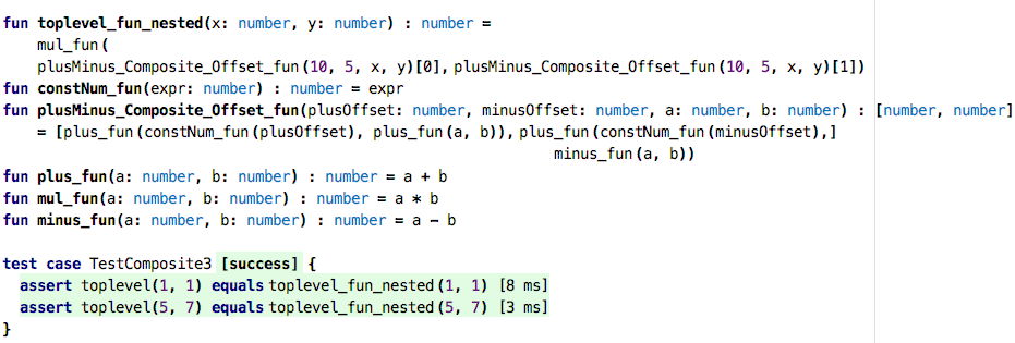
Admittedly, this does not look much better, in fact, you could justifiable argue that it is less readable. In practice it would be a bit different, since the basic blocks and their functions (for plus, minus, etc.) would be predefined somewhere, so we can mentally remove them. What remains isn’t that bad anymore:
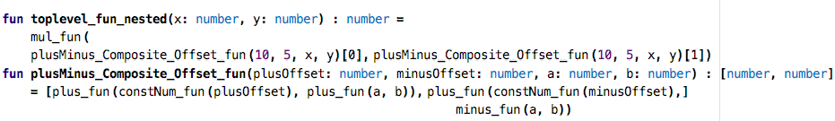
However, once we inline everything, i.e., we get rid of the extra functions and reduce everything to the bare operators, things look different:
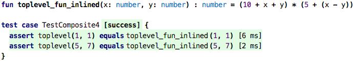
This is really simple now! So what does this tell us? For fine-grained, basic arithmetics, a graphical notation really isn’t worth it. Once things become more involved, and we maybe even have recursion in the computations (shown as cyclic lines in the diagrams), a graphical notation becomes more interesting. And we also learn that dataflow programming is just another form of functional programming as we have seen it before. No big deal!
Function Values
So, what about functions? Can we instantiate functions? Look at this code:
You could say that the function call “instantiates a function”. After all, the
function defines “holes”, i.e., the parameters, and the call provides values.
The problem is that the function call executes right away, evaluates to the
result value (15 and 5 in the example above), and then assigns that value to the val. So the “function instance” created by the call (kind of) has an
infinitesimal lifetime, it never really exists. So, can function calls
themselves (not the thing they evaluate to) be values? Let’s see.
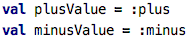
In this code we create two vals, and they represent a value :plus and
a value :minus, respectively.
The colon operator here creates a reference to a function. That reference
is a value, that value can be passed around and modified, like any other value.
What is the type of that value? Let’s ask the tool to automatically annotate
the types:

What we see here are function types, i.e., types that represent functions. The
type given here is the type of functions that take two numbers as arguments
and produce another number. Both plus and minus conform to this type; they
take two numbers and produce another one.
What can we do with these values? One thing is that we can execute the functions, by passing values:
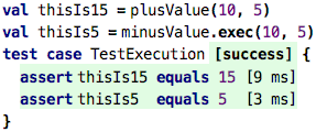
Executing a function directly is exactly the same as executing a value that contains
a reference to that function. You can even use the same ()-based syntax (as shwon
in the thisIs15 example), alternatively you can also use an explicit call to
exec.
However, we can do other neat things. For example, as it is typical for instances, we can provide values for parameters, even without executing them at the same time. This is similar to the configuration parameters in the data flow example shown above. Consider the following:
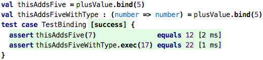
Using bind, you specify some of the parameters of a function call (a process
called partial application). So what happens here is that we use the plusValue (which
is a reference to that original plus function that takes two numbers and
produces a third one) and bind the first argument to 5. This results in a new
function value that now only takes one argument (the first one was just bound
to 5) and adds 5 to that argument. We store this new function value
in the val named thisAddsFive. The type, as we see in
thisAddsFiveWithType is now a function that takes one number and produces
another one. As the tests show, we can now use this value as a function with one
argument, a function that adds 5 to whatever we pass in.
So, if these things are values, we should be able not just to store them in vals,
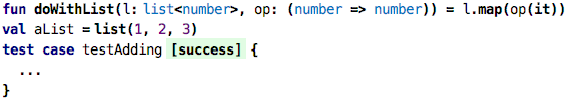
but also to pass them around, right? Absolutely:

Check out the function doWithList. It takes two arguments. The first one
is a regular list of numbers. The second is a function that takes a number
and produces a number (like the thisAddsFive we just created). The idea of doWithList is that is produces a new
list, where the function we pass as the second argument is applied to all
elements of the list we pass as the first argument. We implement this
function using the map operator on the list which we have seen before.
So do you realize what we have just done? We have implemented our own version
of map! We can rename the function and make it an extension function, then
we can literally use them in identical ways:
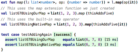
Well, not quite identical. In the native case we explicitly execute the
thisAddsFive function value with the it that represents the list’s
element we currently iterate over. In the case that uses our own map
extension function we just pass a function value. Can we simplify this?
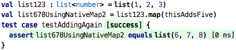
Indeed we can. So what do these higher-order functions, natively built in
(like map, where, etc.) or built by us exactly do? How do they work? They expect function values, i.e., values of type function type,
as arguments. So going back to
our own higher-order function …
… how can we construct valid values for the second argument? Here are three ways:
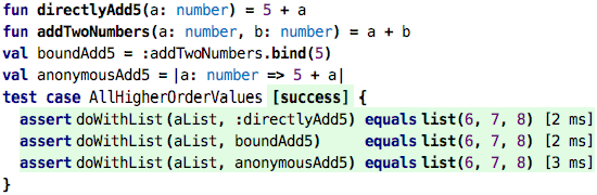
We can pass a reference to a function whose signature is compatible (first test), we can pass one whose signature has been made compatible through partial application (second test), and we can pass a value that represents an anonymous function. We have not really seen those before, so let’s close with explaining these.
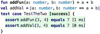
So the anonymousAdd5 value is what we call a lambda expression, or an anonymous
function. It defines one argument, a: number and then has a body that adds 5 to
that a. The lambda itself has no name, but it doesn’t need one, because we
assign it to a val. The following two are essentially equivalent:
The latter has the advantage that you can define it also in places other than the top level of a program that contains functions, records or test cases. You can, for example, define it inside a function …
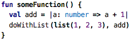
… or anonynously, in a call:

The map on collections is typically used with anonymous function values:
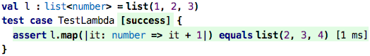
Because these one-argument anomymous lambdas are extremely common with collections (because one wants to process each element, iteratively), there is a short form for the lambdas that can only be used with these higher-order collection operations. The following code is identical to the previous one:
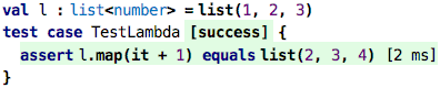
Here, the argument is automatically named it, and it is automatically typed
with the element type of the collection on which map or where is called.
Wrap up
So this brings us full circle: we have just explained higher-order functions and the lambda expressions we have used before via instantiation. This finishes the second part of the tutorial. Part three, once written, will deal with stateful programs and the passage of time.