Go back to Collections
Chapter 07: Decisions and Calculations
In the end, programming is about performing calculations and making decisions, often interleaved. To be able to make these, we need data structures (as we have explained in the previous two chapters) and ways of expressing behavior (expressions and functions, as introduced even earlier). Once the decisions and calculations become more complicated, it becomes important how we represent these decisions to keep them understandable to ourselves and other people who might want to read and understand them. A really important ingredient is to choose appropriate abstractions. I will provide some ideas in this chapter.
Mathematical Notations
Remember the midnight equation from school? I actually didn’t, and I had to look it up :-) But I did remember that it uses a few mathematical notations that serve as a nice demo here. So here is the midnight equation, packaged into a function:
Do you recognize it? Hardly. You can make it slightly better by introducing intermediate values and names, for example, like this:
But you still have to work on recognizing it. A much better representation of the formula is this:
In KernelF, the language we use for this tutorial, you can actually write the formula exactly like this, and you can execute it; all three versions return the same, at least for one test case:
So why am I showing this? Because it demonstrates how important it is to select the right notation. All three representations of the formula do exactly the same thing. Moreover, they use exactly the same abstractions: multiplication, subtraction, division, and so on. The only difference is the way these abstractions are represented in terms of the symbology used.
There’s of course one detail that has been missing (did you notice?): the midnight equation has two results, the plus in the numerator can also be a minus. You could implement this by returning two values, modularizing the calculation accordingly:
The return type is now a list, and you would have to take that into account when working with the return value. Another approach would be to change the function so that you can tell it whether to compute the first or the second solution:
However, in all of these cases, the use of the mathematical notation really makes things much easier to read and understand. So, if you are involved with designing a DSL, make sure you properly motivate the language designers to use nice notations. It’s not just “cosmetics”!
You might ask: what’s the big deal? Of course it is a good idea to use the native mathematical notation to represent mathematical things. And yes, this is true. But mainstream programming languages (those not optimized for math, like Mathematica) can only use sequential text as part of their syntax. So the version that uses root symbols and fractions bars is simply not possible. KernelF, the language we use in this tutorial, relies on MPS, which supports essentially arbitrary notations, including the math symbols shown here, but also including all the other non-textual stuff shown in this and the next chapter.
Complex Decisions
Single Dimension: In the last example, we have seen a very simple decision: based on whether
the caller of the function wanted the first or second solution, we compute
a sign value using an if expression. We have seen if before: if the
Boolean value behind the if, the condition, is true, the overall if
evaluates to the then value; otherwise it evaluates to the else value.
If, therefore, is a way to make a decision between two alternatives.
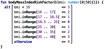
Another way of writing the same decision is by using the alt expression:
However, the alt expression can be used to decide between more than two alternatives.
Below is an example that returns a risk factor based on somebody’s body
mass index:
As you can see, we use several alternatives that cover the range of values
of the body mass index, and depending on the amount of over- and under-weight
we assign a risk factor (this is not a real medical example, I made this
up based on other risk classifications I know from medical projects!).
If we were to write this with ifs, we could do this by nesting; here is the corresponding
code:
However, it’s really hard to read. The alt syntax is much better.
But there are more improvments possible. For example, the repetition of numbers is a problem.
There are several ways
to make this more readable. First, we can use the inRange operation:
This is a little bit more compact but still kinda verbose (notice the [
on the upper limit to express that it’s < instead of <=). One reason
why this is still verbose is that we have to repeat the bmi.inRange again
and again. The reason for this, in turn, is that we could write all kinds
of Boolean expression here; for example, we could take into account the
age of the person:
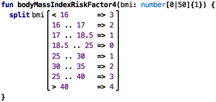
It’s very obvious that this will get out of hand quickly, and we will get back to this case later; for now, let us look at another way of splitting a single range, such as the BMI:
Note how we use split instead of alt. The split expression is explicitly
designed to break down one value
into subranges; this is why the value, bmi, is pulled before the various
cases and does not have to be mentioned in each case. On the flip
side, you cannot add a second value, such as the age from the example above.
It is a nice example how it is useful to have a special-purpose expression
to handle a (presumably) common problem in a way that is much more readable
than using a more general-purpose concept like alt.
Two Dimensions: As we have seen above in the example with bmi and age, you often
have to make a decision based on two criteria; the risk factor involved
in somebody’s weight depends also on their age. Here is a two-dimensional decision table that
represents such as decision:
This decision table evaluates to the number in the (content) cell depending on which column and row headers evaluate to true:
A note on the notation: even though it uses a tabular notation like the spreadsheets we have seen before, the semantics, i.e., the meaning, is different: it’s not just a collection of “cells with values”. Instead, the row and column headers are required to be Boolean expressions, and the result of the evaluation of the overall table is a single value.
Instead of using this tabular notation, one could represent this decision
as nested alt expressions. However,
because the two dimensions are independent and (potentially) every
combination has a different risk, this becomes very hard to read quickly. It is the same
argument that we also made when justifying the alt expression relative to nested ifs.
More Dimensions: Sometimes decisions depend on more than two independent dimensions. Since
we cannot sensibly represent a 5-dimensional table, we need a different mechanism. So let’s introduce
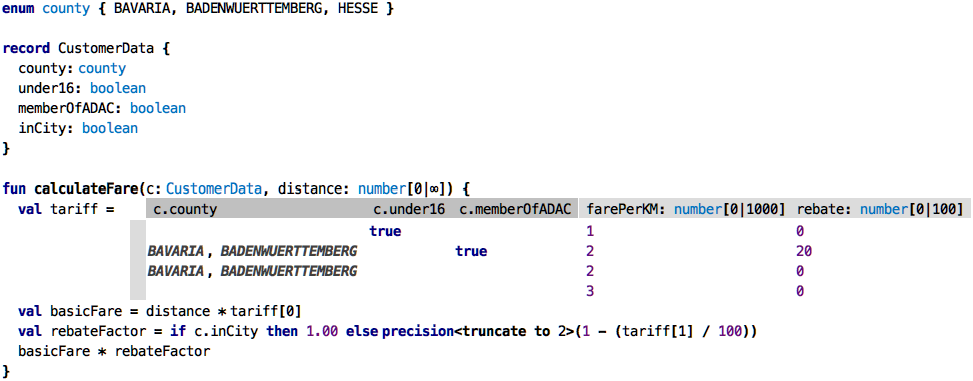
our multi-decision tables. They work as follows: first, they are evaluated in row order, top-down. Rows
that are mentioned earlier are matched first. Each of the colums is matched by ==,
the columns in each row are and‘ed together. If a cell contains comma-separated
values, these count as an or. As an example, we use a fictional computation of a train fare;
these are notoriously complicated.
The overall function takes a CustomerData for matching against the table; we’ll discuss this
below. The table returns two values, packaged into a tuple, accessible positionally via the
square brackets. So the total price for the distance travelled is the product of the baseFare
and the distance. We then compute an rebateFactor; if you are within a city (“Nahverkehrsverbund”),
you get no rebate, the factor is 1.00, else it is computed from the given rebate percentage.
Finally, we compute the resulting fare by multiplying the distance-dependent basicFare by the
rebate factor.
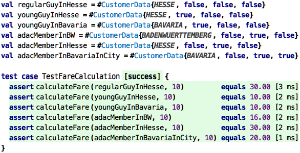
So, to illustrate how this table works, let us work through a couple of test cases:
regularGuyInHesse: None of the specific lines matches, so it “falls through” to the last line, resulting in a fare of 3, multiplied by 10 km, means 30.00.youngGuyInHesse: here, the first line matches, since it has no state constraint. We pay 10.00.youngGuyInBavaria: here, also the first line matches, for the same reason.adacMemberInBW: here we match the state, plus theadacMemberflag; resulting in line 2. So this would a km price of 2, with 20% rebate.adacMemberInHesse: there is no ADAC rebate in Hesse, so they pay the regular price of 3 per km.adacMemberInBavariaInCity: Being in a city invalidates all rebates, so that guy pays the regular Bavaria price of 20.00.
Consistency Checking
While the tables are better than a whole bunch of nested ifs or alts, it might still be hard
to get them correct. For example, in the bodyMassIndexRiskFactorWithAge above, there is a bug:
in the last line, it should say age >= 50 and not just >. The current table does not handle
the case where age == 50: we say the table is incomplete. How can we find such errors? Of course
we can test. But if we don’t happen to test for age 50, we won’t find the problem (remember the discussion on coverage in the context of testing?). Is there a better way?
Yes, there is. Because we have expressed it as a decision table, and because, by definition,
decision tables have to be complete, we can use a so-called solver to check this completeness.
If we apply the solver to that table, it reports:
Error: Missing Row. For instance,
the following case is not covered: age = 50.
A solver tries to proof that for all possible values, the table has a result. If it finds an
example for which this is not the case, it reports this example. It reports such an example
to the user as an error; age = 50 is such an example.
Here’s another one with a bug. See it?
The solver marks lines three and four and reports:
Error: Overlapping Rows: These rows all match in the following case: age = 35
Here we have a non-uniqueness: an age of 35 matches two lines, so the table cannot uniquely decide. So overlap-freedom is another aspect of correctness that the solver can automatically check. One more:
Is this one correct? Notice how we now check the bmi only for values greater than 10,
and we never check any age greater than 120. Why is this not an error? Because the
variables bmi and age have range limits, expressed in the function signature. So, when
checking the table for completeness and consistency, the solver of course takes into account
what values are possible in the first place, based on constraints expressed in other places
in the program. If we were to decide that we now allow for a BMI less than 10 or for ages greater
than 120, and we adapted the types in the functions accordingly, the solver would start reporting
errors.
We use the solver also to verify the multi-decision tables (the fare example). Here, we
check that a line does not shadow lines further down, because then those would never ever
be selected. We also check for completeness and consistency in alt expressions. Generally,
solvers can find many non-trivial bugs.
Solvers are sophisticated tools not typically used in programming languages to find errors. One reason for not using them is that many languages lack the languages features based on which solvers can be applied in a way that lead to meaningful error messages. Also, integrating a solver completely with a language is a lot of work, as we are currently experiencing :-)
Recursion
Let’s say you’re a little child. You want to add two numbers. But the only thing you can do,
in terms of your math expertise, is to add one to a number or substract one. Now let’s also
imagine you are a little child who can write code :-) How would you implement adding two numbers
when you only know how to add or subtract one? Here is what we have initially; the tests fail,
of course, since we just return zero from our add function.
The plus1 function is your low level mechanism to add one to a number, minus1 is the low-level subtraction. The add function should now be implemented by only using plus1. So let’s look at an implementation that actually works:
So what is happening here? Let’s say we want to add 3 + 3. We can rewrite
this as (3 + 2) + 1, where we have introduced one of our basic operations
+1 that we know how to do. 2, in turn, is of course 3 - 1, which uses
the other thing we know how to do, subtracting one. So we are at
3 + 3 ==> (3 + (3 - 1)) + 1
which means that we have sucessfully removed every operation except plus
and minus one. Here is the key observation: how can we compute
(3 + (3 - 1))? We can simply invoke add again. If we expand the complete
calculation, we get
add(3, 3)
    ==> add(3, 2) + 1
            ==> add(3, 1) + 1 + 1
                    ==> add(3, 0) + 1 + 1 + 1
                            ==> 3 + 1 + 1 + 1
                                ==> 6
                        6
                6
        6
6
A function that calls itself with
other arguments is called recursive. A recursive function must at some
point stop calling itself, otherwise the program will run forever.
In our case, when we call add with the second
argument as zero, we know that there’s no more work to do and we can
just return the first argument, without calling add again. This is why
we use the alt expression
in the function to distinguish the recursive case from the base case.
Recursion is not so easy to understand. Many programmers, including myself, have problems understanding it once its use becomes more involved than in this example. I would think that you will likely not use it much. But it is useful to know about. Sometimes it is indeed used even by people who are not necessarily programmers. Take a look at the following code:

Notice how the
l function calls itself with a different value for the variable x.
And yes, this is code! It looks like a Word document, which is intended:
these recursive formulas were found in a Word document that defines recursive,
numerical functions in actuarial math in insurances. We have built a language
that resembles the Word notation as closely as possible.
Debugging and Tracing
As decisions and calculations become more complex, there will be errors. To find those, you have to understand what is actually going on. In spreadsheets, this is relatively easy, because one of a spreadsheet’s nice features is that cells can also output values: if you switch a spreadsheet into the respective mode, cells contain the values to which the expressions in that cell evaluate. This makes a computation “visible”. As usual, the example below shows the spreadsheet in its evaluated version on the right:
If we move outside spreadsheets, how can we understand a program’s internal behavior?
vals and functions and if expressions and the like are not spreadsheet cells, so
how can we see their value?
Tests: We have already seen one way: we can write assertions in test cases. Consider
the following test (testing our previously developed recursive add function):
We can see the values which a particular expression (here: the call to add) evaluates to.
If our expecation is not met, the system outputs the alternative actual value. This works,
but it has two limitations. One, it’s quite a lot of code we have to write just to see
the value of an expression. And second, we can only look at values that are somehow
addressible. For example, we can’t use this approach for an expression inside
a function, because we cannot address it from a test case; it is hidden inside the
function.
Value Inspectors: Let’s go back to one of our initial examples:
How can we understand better what the results are? Can we somehow peek into the values
spd1 and spd2? The easiest way to do this is to attach a value inspector to the
expressions:
You attach a value inspector using an intention on any expression, i.e., by opening the intentions menu via
Ctrl-Alt-Enterand then selecting theAttach Value Inspectorintention. To actually see a value in the value inspector (as opposed to two empty brackets), you have to evaluate the expression on which it is attached. So, for the inspector on the vals, you might want to write a test that refers to theval.
A value inspector can be attached to any expression, and, if through whatever means,
this expression is evaluated, the inspector shows that value. In the example above, we
have attached the inspector to the initialization expressions for the two vals.
You can also look inside a function:
Note how here, the inspector shows two values for the two expressions each (separated
by a comma). Why is this? It is because the function speed was called twice, and the
inspector records all the values, and outputs all of them.
So, while this works for simple cases, we ultimately need a more sophisticated way of tracing computations; we’ll introduce one in the next subsection, but before we do this, I want to briefly close the loop with spreadsheets; you can use the inspector in those too, to peek inside parts of expressions inside spreadsheets, even hierarchically:
The Computation Trace: The value inspectors shown above work nicely for simple
cases. But they also have drawbacks: you have to attach the inspectors manually to all
nodes whose value you want to inspect. And if the same program node is executed several
times (as in the case of the function body of the speed function), the comma-separated
list of values is not a very good solution in general. Enter the tracer.
Let us recap how the execution of a functional program works. A functional computation is
essentially a tree: if you evaluate an expression, then, as part of the evaluation, all
expressions on which the current one depends are evaluated first. So, if we evaluate a + b
where a and b are references to vals, then the first step is to evaluate
a and b before we perform the actual addition. So, here’s the idea: we can display any
function computation as a tree. Let’s check this out with a Hello World:
Here is the computation tree:

To create the trace, select a
valor anassertand pressCtrl-Alt-Shift-Enter(like the key combo for evaluation, but withShift).
If you look at the tree, you can see that, for each of the program nodes, there is a tree node that shows
- the program node’s syntax (e.g.,
val a) - and the value (e.g.,
=> 1) - the type of the value (e.g., Java’s
: BigInteger) - as well as the language construct (e.g.,
[NumberLiteral])
By default, the tree is collapsed, and you can explore the computation by opening successive
tree nodes. Let’s see what happens if the same program node is evaluated several times, a problem
with the earlier value inspector mechanism. In this example, the add function is called three
times in total:
If you look at the trace tree, you can see that the add function shows up three times, but
each time evaluates to a different value. So, importantly, the tree has a node for each
evaluation of a program node, not just for each program node. The same program node (e.g., add)
can show up several times in the trace tree (e.g., for each call to add).

Now, seeing the execution as a tree that is separate from the program source can make it hard to relate that tree to the program. For this reason, you can double-click on any tree node and highlight the values of that node and all its children directly in the code:

The tracer has many more features, such as marking a program node in the code and automatically highlighting it in the trace, jumping from one evaluation of a particular program node to the next evaluation of that same node, and various ways of filtering the level of detail of the tree.
Continue with Instantiation


